Excel Tips: How to Cut Down on Calculations Using SUMIF and SUMIFS
The SUMIF and SUMIFS function in Microsoft Excel is a simple, yet powerful calculation tool. This tutorial will show you how this function works, as well as provide examples of how to use it. Most of you are aware that the SUM function calculates the total of a cell range. SUMIF takes this calculation step a bit further. It says, “Only SUM the numbers in this range IF a cell in this range contains a specific value.”
SUMIF Arguments: Range, Criteria, and Sum Range
Proper syntax: =SUMIF(range, criteria, sum_range) Range and criteria are essential parts of any SUMIF equation; while the sum range is optional. What does each part do, in English?
- Range - The range of cells you want Excel to search. This could be a block of cells, in which case you would use the top left corner and bottom right corner of your range (A1:C3, for example, gives a three by three area of cells).
- Criteria - Defines the flag Excel is to use to determine which cells to add. Using our spreadsheet example below, the criteria could be “Non Edible”, “October” or “Car”, to name a few. In many cases, it’s just a number. It could be greater than, less than, or equal to, as well.
- Sum Range - Optional. Defines the cells to sum. This range holds the actual numbers. If it’s left out of the equation, the function sums the range. As with range, this could be a block of cells, column or rows.
Using the SUMIF Function
For this tutorial, we’re going to use a simple table to track household expenditures for two months. To set up your table and criteria, you first have to define the overall goals. In this example, our goals are:
- determine monthly household costs
- provide a breakdown of overall costs
- automatically update of calculations Let’s get started!
(1) Spreadsheet Setup
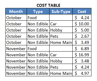
Create a table called COST TABLE with the following headings: Month, Type, Sub-type, and Cost. Fill them in, as shown in the screenshot below:

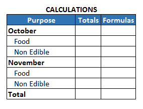
Create a table called CALCULATIONS, and add the following headings in the first column: October, Food, Non Edible, November, Food, Non Edible, and Total - following the format below:

(2) Write the SUMIF Function in the CALCULATIONS table
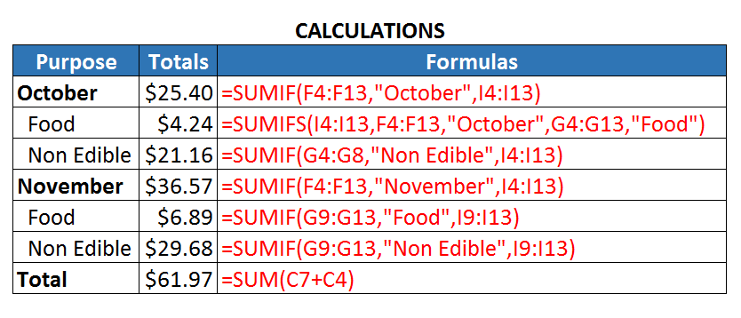
The SUMIF function in C4 (column C is the Totals column) totals the Cost column depending on the Type of the entry. Cell C4 says: SUMIF(the Month column, equals October, add the Cost column) - =SUMIF(F4:F13,”October”,I4:I13)
Meanwhile, the formula for cell C5 - =SUMIF(G4:G8,”food”,I4:I8)
Notice how the range only goes from G4:G8, as I only want to total food for October. If wanted to total food for November as well, I’d use the range G4:G13. Now, if the Month column was not sorted, then I’d need to use the SUMIFS function and specify to criteria - e.g., =SUMIFS(I4:I13,F4:F13,”October”,G4:G13,”Food”)
This produces the exact same results - $4.24. The syntax is slightly different in that you specify the sum_range first, and it is mandatory. _ Proper syntax:_ =SUMIFS(sum_range, criteria_range1, criteria1, criteria_range2, criteria2, criteria_range3, criteria3 …)

(3) ** **Automatic Updates
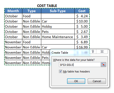
In order for the calculation table to update when a number is changed or when a new row is added, you need to change the COST TABLE from a range to an actual table. To do that in Excel, click anywhere in the table and press Crtl+T on your keyboard. Make sure you do not include the COST TABLE label in your range selection:

Now, you’ll need to rewrite your functions. For example, cell C4 will now be - =SUMIF(Table1[Month],”October”,Table1[Cost])
See the difference? Instead of the range, there is the table name and header. Update all of the functions to match this syntax:

Now when you make any changes the CALCULATIONS table will update automatically (compare the two Totals columns to see the changes). Click here to watch the video.
(4) More Examples
SUMIF can use criteria such as greater than or less than. For example, if you only want to total costs larger than $4, you can write:
Example 1: =SUMIF(I3:I12,”>4”,I3:I12)
SUMIF functions can be written without the sum range if it’s the same as the range. In the example below, we’re telling Excel, “Sum any values greater than 4 in the Cost column.”
Example 2: =SUMIF(I3:I12,”>4”)
If the criteria is a number or cell reference, the function can be written without quotes. If the criteria is an expression or text, frame it in quotes.
Example 3: without quotes, if the range equals the value in cell I3: =SUMIF(I3:I12, I3)
Combine SUMIF with other functions for higher calculations, such as summing and then dividing, by placing the entire function in parenthesis:
Example 4: =SUM ( (SUMIF (I3:I12,”>4”) ) /3 )
Tip: Remember that Excel calculates using the standard order of operations.
The Benefits of SUMIF
SUMIF has many benefits, but a big bonus is the ability to limit the number of spreadsheets. By adding defining columns rather than using spreadsheets (a Month column instead of splitting October costs and November costs into separate sheets, for example), you keep all the data on a single sheet. In turn, it becomes easier to sort, compare, and modify groupings. Now, when you add to your Cost Table, your calculations will automatically update. All you have to do is type your entries. Try it yourself!